


A marketing manager promises a new website by May 1. She lists the tasks in a spreadsheet, adds up the days and feels safe. Two weeks in, the designer is waiting on wireframes, the developer is waiting on design and May 1 is gone. The task list was right. What it could not show was which tasks had to wait for which.
A Gantt chart shows that at a glance: each task as a bar on a calendar, so overlaps, gaps and dependencies are visible. This guide builds one for a real-sized project in Excel and Google Sheets, then uses it to find the tasks that actually decide the deadline.
Why Planning Time Pays Off
Oxford professor Bent Flyvbjerg and Alexander Budzier have studied more than 22,000 projects across 126 countries. In their data, only about 8% met both budget and schedule targets. Typical projects spend about 3% to 5% of total cost on planning, while the best performers spend about 20% to 30%. A Gantt chart is one of the cheapest planning tools available, and it makes the schedule argue back before the work starts.
The Example Project
An invented eight-task website redesign starting Monday, April 6, 2026. Durations are in calendar days to keep the math simple.
| # | Task | Depends on | Start | Duration (days) | End |
|---|---|---|---|---|---|
| 1 | Kickoff and goals | None | Apr 6 | 2 | Apr 7 |
| 2 | Content audit | 1 | Apr 8 | 5 | Apr 12 |
| 3 | Sitemap and wireframes | 2 | Apr 13 | 6 | Apr 18 |
| 4 | Visual design | 3 | Apr 19 | 8 | Apr 26 |
| 5 | Copywriting | 2 | Apr 13 | 10 | Apr 22 |
| 6 | Development | 4 | Apr 27 | 12 | May 8 |
| 7 | Content entry and testing | 5, 6 | May 9 | 5 | May 13 |
| 8 | Launch and redirects | 7 | May 14 | 1 | May 14 |
Use a formula for the end date instead of typing it: End = Start + Duration − 1. And make each start date depend on the task before it, for example Start of task 3 = End of task 2 + 1. Then, if one task slips, every later date moves automatically.
Building It in Excel
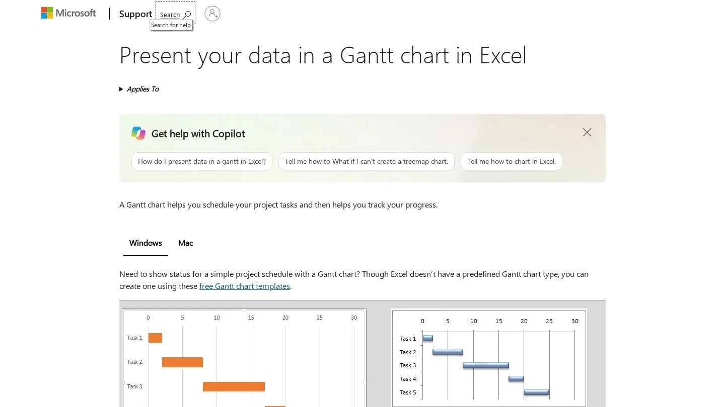
Excel has no built-in Gantt chart, but a stacked bar chart does the job.
- Set up three columns: Task, Start and Duration.
- Select the three columns and choose Insert, then Bar Chart, then Stacked Bar.
- Hide the first series. Click the bars for Start, then set Fill to No Fill and Border to No Line. The Duration bars now float at the right dates.
- Reverse the task order. Right-click the vertical axis, choose Format Axis and tick “Categories in reverse order,” so task 1 sits at the top.
- Fix the date axis. This is the step most tutorials skip. Excel starts the horizontal axis at zero, which is January 1900, so your bars sit far to the right of a mostly empty chart. Right-click the horizontal axis, choose Format Axis and set the Minimum to the serial number of your start date. April 6, 2026 is 46118. Type =DATEVALUE(“2026-04-06”) in any cell and format it as a number to find the serial for any date.
- Set the major unit to 7 so gridlines appear weekly.
- Color the critical path differently, as explained next.
Building It in Google Sheets
Google Sheets offers two routes.
Option 1: Timeline View
On paid Google Workspace plans such as Business Standard and above, select your table and choose Insert, then Timeline. Sheets draws the bars from your start and end dates, and you can group them by owner or status. Google says timeline view is not available on personal Google accounts, nonprofit plans or legacy G Suite editions.
Option 2: Conditional Formatting, Which Works on Any Account
- Put your task table in columns A to D, with Start in column B and End in column D.
- In F1, enter the project start date. In G1, enter =F1+1 and copy it across for as many days as the project runs, here about 40 columns.
- Select the grid from F2 across and down to the last task.
- Choose Format, then Conditional formatting, then “Custom formula is,” and enter: =AND(F$1>=$B2, F$1<=$D2)
- Pick a fill color. Each task now shows as a colored bar across its dates.
- Narrow the date columns and format the header as day and month to make it readable.
This version updates instantly when dates change and works in Excel too, using the same formula in Excel’s conditional formatting.
Finding the Critical Path
The critical path is the longest chain of dependent tasks. It sets the earliest possible finish date, and any delay on it delays the whole project.
In the example, two chains lead to task 7:
- Design chain: Kickoff (2) → Audit (5) → Wireframes (6) → Design (8) → Development (12) → Testing (5) → Launch (1) = 39 days
- Copy chain: Kickoff (2) → Audit (5) → Copywriting (10) → Testing (5) → Launch (1) = 23 days
The design chain is the critical path. Copywriting finishes on April 22 but is not needed until testing starts on May 9, so it has 16 days of slack. A copywriter running a week late changes nothing. A designer running two days late moves launch by two days.
What the manager should have done: With a May 1 deadline and a 39-day critical path from April 6, the plan was late before it began. The options were to start earlier, shorten development by adding a developer, or run design and development in overlapping stages, not to hope.
Dig deeper: Color critical path bars red and the rest gray. In status meetings, discuss red bars first. Gray bars with slack rarely need attention.
Keeping the Chart Useful
- Add a progress column with percent complete, and show it as a second, darker bar or a fill pattern.
- Mark today: In the conditional formatting version, add a rule that highlights the column where the date equals TODAY().
- Add milestones: Zero-day tasks, such as “Client approves design,” shown as a diamond or a bold border.
- Update weekly: A Gantt chart that is three weeks out of date is worse than none, because people trust it.
When a Spreadsheet Is Not Enough
Spreadsheets work well for projects with up to about 30 to 50 tasks and one planner. Consider dedicated tools when you need automatic dependency scheduling, resource loading across several projects, or many people updating tasks at once. Microsoft Project, Smartsheet, Monday.com, Asana, ClickUp and TeamGantt all include Gantt views with dependencies built in.

Frequently Asked Questions
Does Excel have a Gantt chart template?
Yes. Excel includes Gantt project planner templates under File, then New. They use conditional formatting rather than a chart, and work well for simple projects.
How do I show dependencies in an Excel Gantt chart?
Excel charts cannot draw dependency arrows automatically. Link start dates with formulas so later tasks move when earlier ones slip, and note dependencies in a column. For drawn arrows, use a project management tool.
Should durations be in working days or calendar days?
Working days are more realistic for business projects. In Excel and Google Sheets, use the WORKDAY function, for example =WORKDAY(B2, C2-1), to calculate end dates that skip weekends, and add a holiday list as a third argument.
What is the difference between a Gantt chart and a timeline?
A timeline shows key dates and milestones along a single line. A Gantt chart shows each task as a bar with its start, duration and overlap with other tasks, which makes it better for planning the work itself.